Fine-tune natural language processing models using Azure Machine Learning service
In the natural language processing (NLP) domain, pre-trained language representations have traditionally been a key topic for a few important use cases, such as named entity recognition (Sang and Meulder, 2003), question answering (Rajpurkar et al., 2016), and syntactic parsing (McClosky et al., 2010).
The intuition for utilizing a pre-trained model is simple: A deep neural network that is trained on large corpus, say all the Wikipedia data, should have enough knowledge about the underlying relationships between different words and sentences. It should also be easily adapted to a different domain, such as medical or financial domain, with better performance than training from scratch.
Recently, a paper called “BERT: Bidirectional Encoder Representations from Transformers” was published by Devlin, et al, which achieves new state-of-the-art results on 11 NLP tasks, using the pre-trained approach mentioned above. In this technical blog post, we want to show how customers can efficiently and easily fine-tune BERT for their custom applications using Azure Machine Learning Services. We open sourced the code on GitHub.
Intuition behind BERT
The intuition behind the new language model, BERT, is simple yet powerful. Researchers believe that a large enough deep neural network model, with large enough training corpus, could capture the relationship behind the corpus. In NLP domain, it is hard to get a large annotated corpus, so researchers used a novel technique to get a lot of training data. Instead of having human beings label the corpus and feed it into neural networks, researchers use the large Internet available corpus – BookCorpus (Zhu, Kiros et al) and English Wikipedia (800M and 2,500M words respectively). Two approaches, each for different language tasks, are used to generate the labels for the language model.
- Masked language model: To understand the relationship between words. The key idea is to mask some of the words in the sentence (around 15 percent) and use those masked words as labels to force the models to learn the relationship between words. For example, the original sentence would be:
The man went to the store. He bought a gallon of milk.
And the input/label pair to the language model is:
Input: The man went to the [MASK1]. He bought a [MASK2] of milk.
Labels: [MASK1] = store; [MASK2] = gallon
- Sentence prediction task: To understand the relationships between sentences. This task asks the model to predict whether sentence B, is likely to be the next sentence following a given sentence A. Using the same example above, we can generate training data like:
Sentence A: The man went to the store.
Sentence B: He bought a gallon of milk.
Label: IsNextSentence
Applying BERT to customized dataset
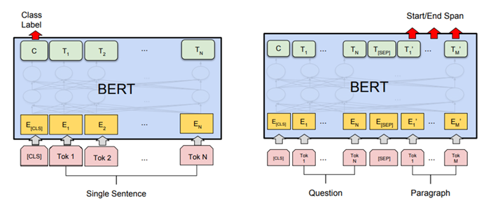
After BERT is trained on a large corpus (say all the available English Wikipedia) using the above steps, the assumption is that because the dataset is huge, the model can inherit a lot of knowledge about the English language. The next step is to fine-tune the model on different tasks, hoping the model can adapt to a new domain more quickly. The key idea is to use the large BERT model trained above and add different input/output layers for different types of tasks. For example, you might want to do sentiment analysis for a customer support department. This is a classification problem, so you might need to add an output classification layer (as shown on the left in the figure below) and structure your input. For a different task, say question answering, you might need to use a different input/output layer, where the input is the question and the corresponding paragraph, while the output is the start/end answer span for the question (see the figure on the right). In each case, the way BERT is designed can enable data scientists to plug in different layers easily so BERT can be adapted to different tasks.

Figure 1. Adapting BERT for different tasks (Source)
The image below shows the result for one of the most popular dataset in NLP field, the Stanford Question Answering Dataset (SQuAD).

Figure 2. Reported BERT performance on SQuAD 1.1 dataset (Source).
Depending on the specific task types, you might need to add very different input/output layer combinations. In the GitHub repository, we demonstrated two tasks, General Language Understanding Evaluation (GLUE) (Wang et al., 2018) and Stanford Question Answering Dataset (SQuAD) (Rajpurkar and Jia et al., 2018).
Using the Azure Machine Learning Service
We are going to demonstrate different experiments on different datasets. In addition to tuning different hyperparameters for various use cases, Azure Machine Learning service can be used to manage the entire lifecycle of the experiments. Azure Machine Learning service provides an end-to-end cloud-based machine learning environment, so customers can develop, train, test, deploy, manage, and track machine learning models, as shown below. It also has full support for open-source technologies, such as PyTorch and TensorFlow which we will be using later.

Figure 3. Azure Machine Learning Service Overview
What is in the notebook
Defining the right model for specific task
To fine-tune the BERT model, the first step is to define the right input and output layer. In the GLUE example, it is defined as a classification task, and the code snippet shows how to create a language classification model using BERT pre-trained models:
model = modeling.BertModel(
     config=bert_config,
     is_training=is_training,
     input_ids=input_ids,
     input_mask=input_mask,
     token_type_ids=segment_ids,
     use_one_hot_embeddings=use_one_hot_embeddings)

logits = tf.matmul(output_layer, output_weights, transpose_b=True)
logits = tf.nn.bias_add(logits, output_bias)
probabilities = tf.nn.softmax(logits, axis=-1)
log_probs = tf.nn.log_softmax(logits, axis=-1)
one_hot_labels = tf.one_hot(labels, depth=num_labels, dtype=tf.float32)
per_example_loss = -tf.reduce_sum(one_hot_labels * log_probs, axis=-1)
loss = tf.reduce_mean(per_example_loss)
Set up training environment using Azure Machine Learning service
Depending on the size of the dataset, training the model on the actual dataset might be time-consuming. Azure Machine Learning Compute provides access to GPUs either for a single node or multiple nodes to accelerate the training process. Creating a cluster with one or multiple nodes on Azure Machine Learning Compute is very intuitive, as below:
compute_config = AmlCompute.provisioning_configuration(vm_size='STANDARD_NC24s_v3',
                                                         min_nodes=0,
                                                         max_nodes=8)
# create the cluster
gpu_compute_target = ComputeTarget.create(ws, gpu_cluster_name, compute_config)
gpu_compute_target.wait_for_completion(show_output=True)
estimator = PyTorch(source_directory=project_folder,
                 compute_target=gpu_compute_target,
                 script_params = {...},
                 entry_script='run_squad.azureml.py',
                 conda_packages=['tensorflow', 'boto3', 'tqdm'],
                 node_count=node_count,
                 process_count_per_node=process_count_per_node,
                 distributed_backend='mpi',
                 use_gpu=True)
Azure Machine Learning is greatly simplifying the work involved in setting up and running a distributed training job. As you can see, scaling the job to multiple workers is done by just changing the number of nodes in the configuration and providing a distributed backend. For distributed backends, Azure Machine Learning supports popular frameworks such as TensorFlow Parameter server as well as MPI with Horovod, and it ties in with the Azure hardware such as InfiniBand to connect the different worker nodes to achieve optimal performance. We will have a follow up blogpost on how to use the distributed training capability on Azure Machine Learning service to fine-tune NLP models.
For more information on how to create and set up compute targets for model training, please visit our documentation.
Hyper Parameter Tuning
For a given customer’s specific use case, model performance depends heavily on the hyperparameter values selected. Hyperparameters can have a big search space, and exploring each option can be very expensive. Azure Machine Learning Services provide an automated machine learning service, which provides hyperparameter tuning capabilities and can search across various hyperparameter configurations to find a configuration that results in the best performance.
In the provided example, random sampling is used, in which case hyperparameter values are randomly selected from the defined search space. In the example below, we explored the learning rate space from 1e-4 to 1e-6 in log uniform manner, so the learning rate might be 2 values around 1e-4, 2 values around 1e-5, and 2 values around 1e-6.
Customers can also select which metric to optimize. Validation loss, accuracy score, and F1 score are some popular metrics that could be selected for optimization.
from azureml.train.hyperdrive import *
import math

param_sampling = RandomParameterSampling( {
         'learning_rate': loguniform(math.log(1e-4), math.log(1e-6)),
})

hyperdrive_run_config = HyperDriveRunConfig(
     estimator=estimator,
     hyperparameter_sampling=param_sampling,
     primary_metric_name='f1',
     primary_metric_goal=PrimaryMetricGoal.MAXIMIZE,
     max_total_runs=16,
     max_concurrent_runs=4)
For each experiment, customers can watch the progress for different hyperparameter combinations. For example, the picture below shows the mean loss over time using different hyperparameter combinations. Some of the experiments can be terminated early if the training loss doesn’t meet expectations (like the top red curve).

Figure 4. Mean loss for training data for different runs, as well as early termination
For more information on how to use the Azure ML’s automated hyperparameter tuning feature, please visit our documentation on tuning hyperparameters. And for how to track all the experiments, please visit the documentation on how to track experiments and metrics.
Visualizing the result
Using the Azure Machine Learning service, customers can achieve 85 percent evaluation accuracy when fine-tuning MRPC in GLUE dataset (it requires 3 epochs for BERT base model), which is close to the state-of-the-art result. Using multiple GPUs can shorten the training time and using more powerful GPUs (say V100) can also improve the training time. For one of the specific experiments, the details are as below:
| GPU# | 1 | 2 | 4 |
| K80 (NC Family) | 191 s/epoch | 105 s/epoch | 60 s/epoch |
| V100 (NCv3 Family) | 36 s/epoch | 22 s/epoch | 13 s/epoch |
Table 1. Training time per epoch for MRPC in GLUE dataset
For SQuAD 1.1, customers can achieve around 88.3 F1 score and 81.2 Exact Match (EM) score. It requires 2 epochs using BERT base model, and the time for each epoch is shown below:
| GPU# | 1 | 2 | 4 |
| K80 (NC Family) | 16,020 s/epoch | 8,820 s/epoch | 4,020 s/epoch |
| V100 (NCv3 Family) | 2,940 s/epoch | 1,393 s/epoch | 735 s/epoch |
Table 2. Training time per epoch for SQuAD dataset
After all the experiments are done, the Azure Machine Learning service SDK also provides a summary visualization on the selected metrics and the corresponding hyperparameter(s). Below is an example on how learning rate affects validation loss. Throughout the experiments, the learning rate has been changed from around 7e-6 (the far left) to around 1e-3 (the far right), and the best learning rate with lowest validation loss is around 3.1e-4. This chart can also be leveraged to evaluate other metrics that customers want to optimize.

Figure 5. Learning rate versus validation loss
Summary
In this blog post, we showed how customers can fine-tune BERT easily using the Azure Machine Learning service, as well as topics such as using distributed settings and tuning hyperparameters for the corresponding dataset. We also showed some preliminary results to demonstrate how to use Azure Machine Learning service to fine tune the NLP models. All the code is available on the GitHub repository. Please let us know if there are any questions or comments by raising an issue in the GitHub repo.
References
BERT: Pre-training of Deep Bidirectional Transformers for Language Understanding and its GitHub site.
- Visit the Azure Machine Learning service homepage today to get started with your free-trial.
- Learn more about Azure Machine Learning service.
Source: Azure Blog Feed