Performance troubleshooting using new Azure Database for PostgreSQL features
At Ignite 2018, Microsoft’s Azure Database for PostgreSQL announced the preview of Query Store (QS), Query Performance Insight (QPI), and Performance Recommendations (PR) to help ease performance troubleshooting, in response to customer feedback. This blog intends to inspire ideas on how you can use features that are currently available to troubleshoot some common scenarios.
A previous blog post on performance best practices touched upon the layers at which you might be experiencing issues based on the application pattern that you are using. This blog nicely categorizes the problem space into several areas and the common techniques to rule out possibilities to quickly get to the root cause. We would like to further expand on this with the help of these newly announced features (QS, QPI, and PR).
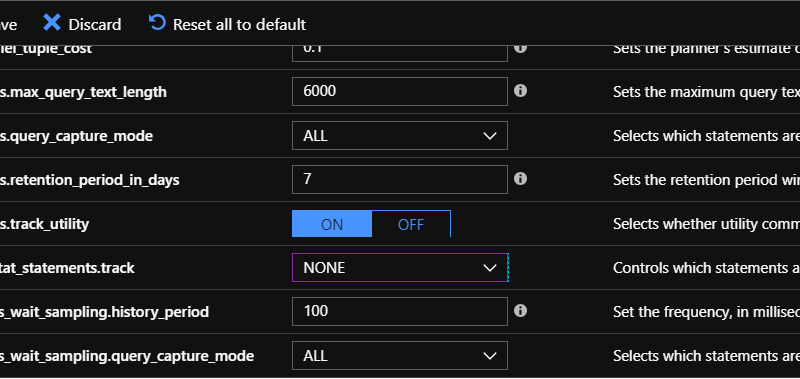
In order to use these features, you will need to enable data collection by setting pg_qs.query_capture_mode and pgms_wait_sampling.query_capture_mode to ALL.

You can use Query Store for a wide variety of scenarios where you can enable data collection to help with troubleshooting these scenarios better. In this article, we will limit the scope to regressed queries scenario.
Regressed queries
One of the important scenarios that Query Store enables you to monitor is the regressed queries. By setting pg_qs.query_capture_mode to ALL, you get a history of your query performance over time. We can leverage this data to do simple or more complex comparisons based on your needs.
One of the challenges you face when generating a regressed query list is the selection of comparison period in which you baseline your query runtime statistics. There are a handful of factors to think about when selecting the comparison period:
- Seasonality: Does the workload or the query of your concern occur periodically rather than continuously?
- History: Is there enough historical data?
- Threshold: Are you comfortable with a flat percentage change threshold or do you require a more complex method to prove the statistical significance of the regression?
Now, let’s assume no seasonality in the workload and that the default seven days of history will be enough to evaluate a simple threshold of change to pick regressed queries. All you need to do is to pick a baseline start and end time, and a test start and end time to calculate the amount of regression for the metric you would like to track.
Looking at the past seven-day history, compared to last two hours of execution, below would give the top regressed queries in the order of descending percentage. Note that if the result set has negative values, it indicates an improvement from baseline to test period when it’s zero, it may either be unchanged or not executed during the baseline period.
create or replace function get_ordered_query_performance_changes(
baseline_interval_start int,
baseline_interval_type text,
current_interval_start int,
current_interval_type text)
returns table (
     query_id bigint,
     baseline_value numeric,
     current_value numeric,
     percent_change numeric
) as $$
with data_set as (
select query_id
, round(avg( case when start_time >= current_timestamp - ($1 || $2)::interval and start_time < current_timestamp - ($3 || $4)::interval then mean_time else 0 end )::numeric,2) as baseline_value
, round(avg( case when start_time >= current_timestamp - ($3 || $4)::interval then mean_time else 0 end )::numeric,2) as current_value
from query_store.qs_view where query_id != 0 and user_id != 10 group by query_id ) ,
query_regression_data as (
select *
, round(( case when baseline_value = 0 then 0 else (100*(current_value - baseline_value) / baseline_value) end )::numeric,2) as percent_change
from data_set )
select * from query_regression_data order by percent_change desc;
$$
language 'sql';
If you create this function and execute the following, you will get the top regressed queries in the last two hours in descending order compared to their calculated baseline value over the last seven days up to two hours ago.
select * from get_ordered_query_performance_changes (7, 'days', 2, 'hours');

The top changes are all good candidates to go after unless you do expect the kind of delta from your baseline period because, say, you know the data size would change or the volume of transactions would increase. Once you identified the query you would like to further investigate, the next step is to look further into query store data and see how the baseline statistics compare to the current period and collect additional clues.
create or replace function compare_baseline_to_current_by_query_id(baseline_interval_cutoff int,baseline_interval_type text,query_id bigint,percentile decimal default 1.00)
returns table(
     query_id bigint,
     period text,
     percentile numeric,
     total_time numeric,
     min_time numeric,
     max_time numeric,
     rows numeric,
     shared_blks_hit numeric,
     shared_blks_read numeric,
     shared_blks_dirtied numeric,
     shared_blks_written numeric,
     local_blks_hit numeric,
     local_blks_read numeric,
     local_blks_dirtied numeric,
     local_blks_written numeric,
     temp_blks_read numeric,
     temp_blks_written numeric,
     blk_read_time numeric,
     blk_write_time numeric
)
as $$

with data_set as
( select *
, ( case when start_time >= current_timestamp - ($1 || $2)::interval then 'current' else 'baseline' end ) as period
from query_store.qs_view where query_id = ( $3 )
)
select query_id
, period
, round((case when $4 <= 1 then 100 * $4 else $4 end)::numeric,2) as percentile
, round(percentile_cont($4) within group ( order by total_time asc)::numeric,2) as total_time
, round(percentile_cont($4) within group ( order by min_time asc)::numeric,2) as min_time
, round(percentile_cont($4) within group ( order by max_time asc)::numeric,2) as max_time
, round(percentile_cont($4) within group ( order by rows asc)::numeric,2) as rows
, round(percentile_cont($4) within group ( order by shared_blks_hit asc)::numeric,2) as shared_blks_hit
, round(percentile_cont($4) within group ( order by shared_blks_read asc)::numeric,2) as shared_blks_read
, round(percentile_cont($4) within group ( order by shared_blks_dirtied asc)::numeric,2) as shared_blks_dirtied
, round(percentile_cont($4) within group ( order by shared_blks_written asc)::numeric,2) as shared_blks_written
, round(percentile_cont($4) within group ( order by local_blks_hit asc)::numeric,2) as local_blks_hit
, round(percentile_cont($4) within group ( order by local_blks_read asc)::numeric,2) as local_blks_read
, round(percentile_cont($4) within group ( order by local_blks_dirtied asc)::numeric,2) as local_blks_dirtied
, round(percentile_cont($4) within group ( order by local_blks_written asc)::numeric,2) as local_blks_written
, round(percentile_cont($4) within group ( order by temp_blks_read asc)::numeric,2) as temp_blks_read
, round(percentile_cont($4) within group ( order by temp_blks_written asc)::numeric,2) as temp_blks_written
, round(percentile_cont($4) within group ( order by blk_read_time asc)::numeric,2) as blk_read_time
, round(percentile_cont($4) within group ( order by blk_write_time asc)::numeric,2) as blk_write_time
from data_set
group by 1, 2
order by 1, 2 asc;
$$
language 'sql';
Once you create the function, provide the query id you would like to investigate. The function will compare the aggregate values between the before and after based on the cutoff time you provide. For instance, the below statement would compare all points prior to two hours from now to points after the two hours mark up until now for the query. If you are aware of outliers that you want to exclude, you can use a percentile value.
select * from compare_baseline_to_current_by_query_id(30, 'minutes', 4271834468, 0.95);
If you don’t use any, the default value is 100 which does include all data points.
select * from compare_baseline_to_current_by_query_id(2, 'hours', 4271834468);

If you rule out that there is not a significant data size change and the cache hit ratio is rather steady, you may also want to investigate any obvious wait event occurrence changes within the same period. As wait event types combine different wait types into buckets similar by nature, there is not a single prescription on how to analyze the data. However, a general comparison may give us ideas around the system state change.
create or replace function compare_baseline_to_current_by_wait_event (baseline_interval_start int,baseline_interval_type text,current_interval_start int,current_interval_type text)
returns table(
     wait_event text,
     baseline_count bigint,
     current_count bigint,
     current_to_baseline_factor double precision,
     percent_change numeric
)
as $$
with data_set as
( select event_type || ':' || event as wait_event
, sum( case when start_time >= current_timestamp - ($1 || $2)::interval and start_time < current_timestamp - ($3 || $4)::interval then 1 else 0 end ) as baseline_count
, sum( case when start_time >= current_timestamp - ($3 || $4)::interval then 1 else 0 end ) as current_count
, extract(epoch from ( $1 || $2 ) ::interval) / extract(epoch from ( $3 || $4 ) ::interval) as current_to_baseline_factor
from query_store.pgms_wait_sampling_view where query_id != 0
group by event_type || ':' || event
) ,
wait_event_data as
( select *
, round(( case when baseline_count = 0 then 0 else (100*((current_to_baseline_factor*current_count) - baseline_count) / baseline_count) end )::numeric,2) as percent_change
from data_set
)
select * from wait_event_data order by percent_change desc;
$$
language 'sql';

select * from compare_baseline_to_current_by_wait_event (7, 'days', 2, 'hours');
The above query will let you see some abnormal changes between the two periods. Note that event count here is taken as an approximation and the numbers should be taken within the context of the comparative load of the instance given the time.

As you can see, with the available time series data in Query Store, your creativity is your limit to the kinds of analysis and algorithms you could implement here. We showed you some simple calculations by which you could apply straight forward techniques to identify candidates and improve. We hope that this could be your starting point and that you share with us what works, what doesn’t and how you take this to the next level.
We are always looking forward to hearing feedback from you!
Acknowledgments
Special thanks to Senior Data Scientist Korhan Ileri, and Principal Data Scientist Managers Intaik Park and Saikat Sen for their contributions to this blog post.
Source: Azure Blog Feed